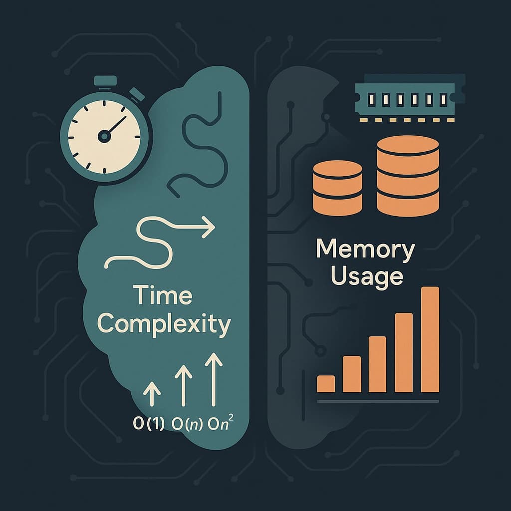
When writing code, the first goal is often to get something working. But once systems grow and traffic increases, the way we handle memory and time complexity becomes critical. These two factors decide whether an app runs smoothly at scale or collapses under pressure.

Ignoring them is like building a city without considering traffic flow. At first, when there are only a few cars, everything seems fine. But as the population grows, poorly planned roads quickly turn into daily gridlock. The same happens with code—inefficiencies that go unnoticed early can become costly bottlenecks later.

Understanding Time Complexity

Time complexity describes how the running time of an algorithm changes as the input size grows. It’s not about exact milliseconds, but about how performance scales.

Big O notation is the language we use to describe how an algorithm’s performance scales as the input grows. Instead of measuring exact seconds or milliseconds, it gives us a way to express the trend, whether the work stays constant, grows linearly, or explodes exponentially. Here are some of the most common complexities:

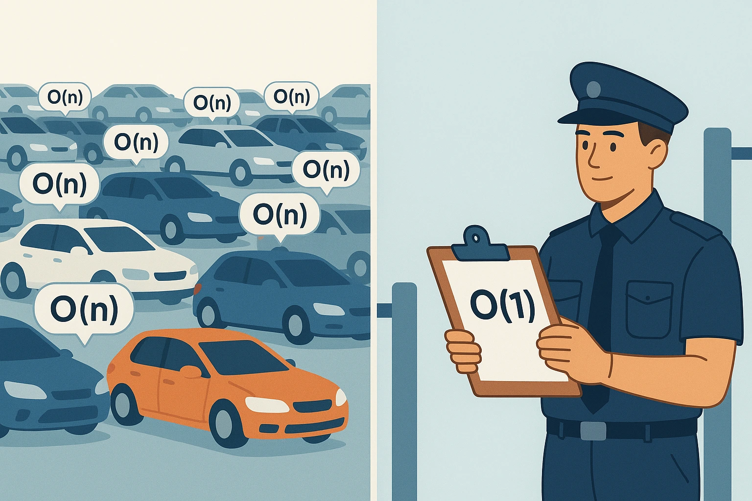
• O(1) – Constant time. No matter how large the input is, the operation takes the same time. Think of finding your seat in a cinema. If your ticket says Row 4, Seat 15, you walk directly to that spot. It doesn’t matter whether the cinema has 100 seats or 1000 — you’re not checking every seat one by one, you already know exactly where to go.
• O(log n) – Logarithmic time. Efficient algorithms like binary search fall here. Imagine guessing a number between 1 and 100 by halving the range each time—you don’t need 100 tries, only about 7.
• O(n) – Linear time. The work grows directly with the input. Reading every guest’s name on a list is O(n). Double the guests, double the effort.
• O(n log n) – Typical for sorting algorithms like quicksort and mergesort. Efficient enough to handle large datasets, but still scales with both size and depth of operations.
• O(n²) – Quadratic time. Comparing every student with every other student in a class to see who shares a birthday. Fine with 20 students, impossible with 20,000.

A practical Go example:

// Linear search: O(n)
func exists(slice []int, target int) bool {
    for _, v := range slice {
        if v == target {
            return true
        }
    }
    return false
}

Versus using a map:

// Hash lookup: O(1)
func exists(m map[int]bool, target int) bool {
    return m[target]
}

Understanding Memory Usage

Memory usage is about the space our code consumes. Each choice of data structure or algorithm has a footprint, and sometimes we trade speed for space—or the other way around.

Example in C:

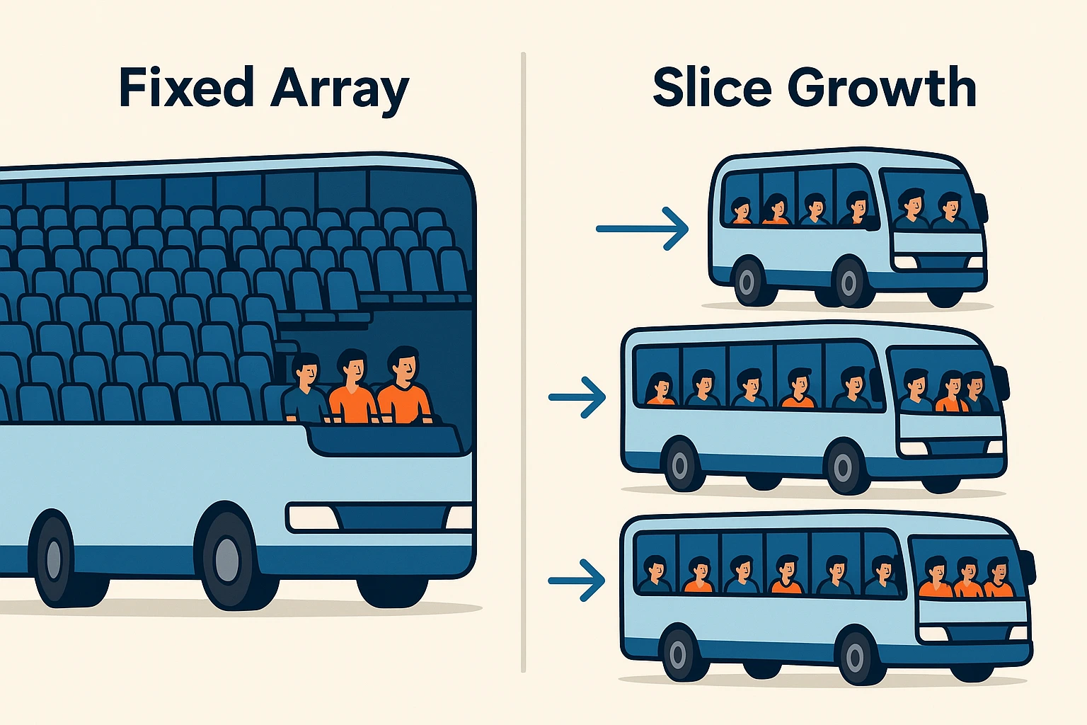
int numbers[1000];

This allocates memory for 1000 integers right away, even if only 10 are ever used. It’s predictable but wasteful. 

In Go, slices handle this differently:

numbers := []int{}
numbers = append(numbers, 42)

Here the slice grows as needed. Under the hood, Go allocates larger chunks (often doubling capacity) to minimize frequent reallocations. That flexibility comes with overhead—more memory is reserved than what’s actually in use. 

It’s like running a bus line:

• Fixed array = sending out a huge bus that might ride half-empty.
• Slice = starting with a minivan, then upgrading to larger buses as demand increases.

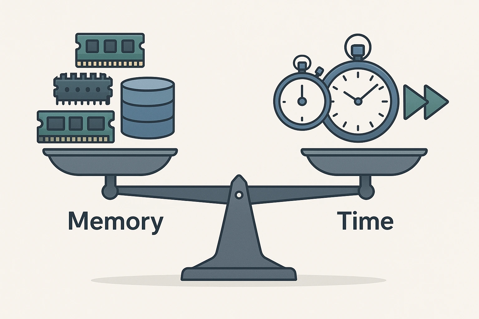
The Balance: Time vs. Memory

Time and memory often work like opposite sides of a scale. Speeding up code may require caching or precomputing results (more memory). Reducing memory usage may mean recomputing values instead of storing them (more time).

A real-world example:

• A social media feed recalculated from scratch (O(n) scan) each time a user logs in is too slow at scale.
• Caching feed results in memory makes retrieval fast but consumes more space.
• The right approach depends on resources, expected traffic, and update frequency.

Why This Matters in Practice

When apps are small, inefficiencies are hidden by modern hardware. But once requests jump from thousands to millions, optimization is no longer optional.

Think of cooking: at home, chopping vegetables slowly with a dull knife is fine. In a restaurant serving hundreds of meals a night, it’s a disaster. Memory and time complexity are the sharp knives of software engineering—they determine whether the kitchen (or system) can keep up with demand.

Wrapping Up

Memory usage and time complexity aren’t academic details. They’re practical levers for building scalable, reliable applications. Every decision, whether to use a slice or a map, a cache or recalculation, a linear search or binary search, comes with trade-offs.

There is no single right answer. The real skill is understanding the trade-offs and choosing the right balance for the problem at hand.